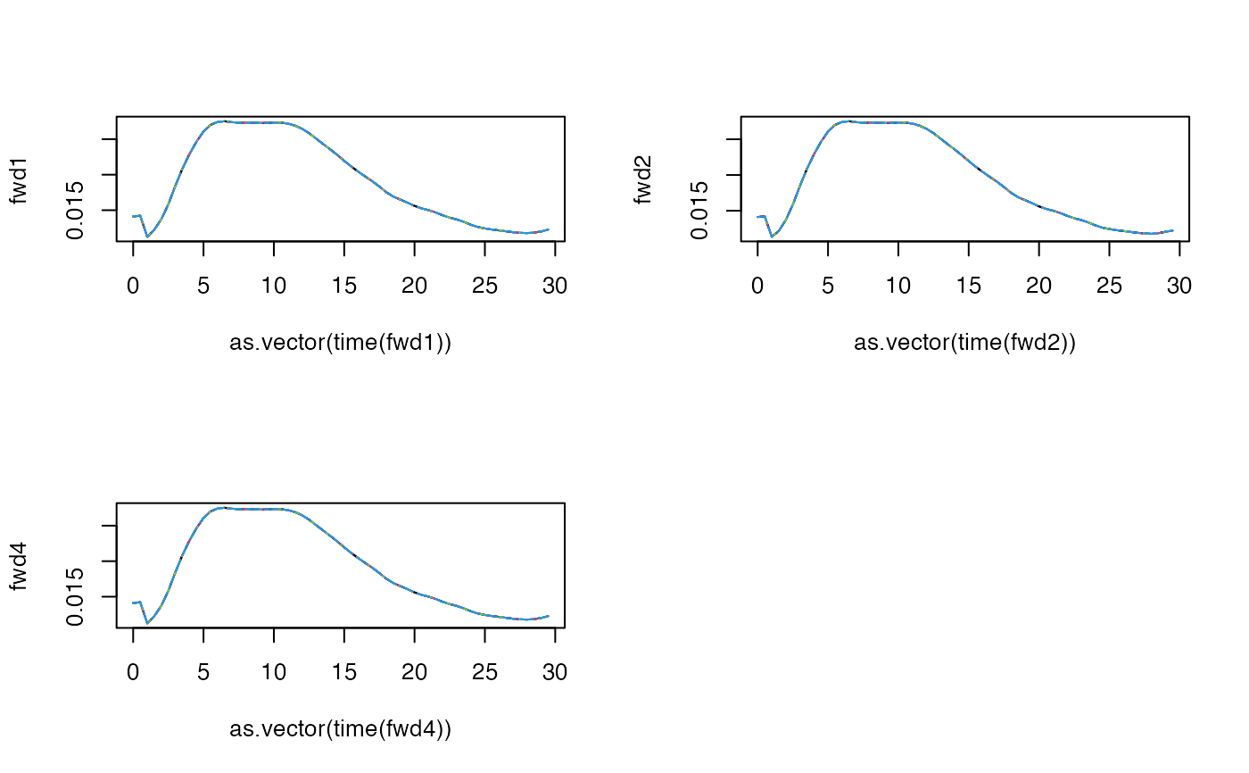
Instantaneous forward rates — esgfwdrates • ESGtoolkit

This function provides instantaneous forward rates. They can be used in no-arbitrage short rate models, to fit the yield curve exactly.

esgfwdrates(
  in.maturities,
  in.zerorates,
  n,
  horizon,
  out.frequency = c("annual", "semi-annual", "quarterly", "monthly", "weekly", "daily"),
  method = c("fmm", "periodic", "natural", "monoH.FC", "hyman", "HCSPL", "SW"),
  ...
)

Arguments

in.maturities: input maturities
in.zerorates: input zero rates
n: number of independent observations
horizon: horizon of projection
out.frequency: either "annual", "semi-annual", "quarterly", "monthly", "weekly", or "daily" (1, 1/2, 1/4, 1/12, 1/52, 1/252)
method: specifies the type of spline to be used for interpolation. Possible values are "fmm", "natural", "periodic", "monoH.FC" and "hyman". See spline; "HCSPL" (Hermite cubic spline) or "SW" (Smith-Wilson)
...: additional parameters provided to splinefun

Author

T. Moudiki

Examples


# Yield to maturities
txZC <- c(0.01422,0.01309,0.01380,0.01549,0.01747,0.01940,0.02104,0.02236,0.02348,
         0.02446,0.02535,0.02614,0.02679,0.02727,0.02760,0.02779,0.02787,0.02786,0.02776
         ,0.02762,0.02745,0.02727,0.02707,0.02686,0.02663,0.02640,0.02618,0.02597,0.02578,0.02563)

# Observed maturities
u <- 1:30

par(mfrow=c(2,2))
fwd1 <- esgfwdrates(in.maturities = u, in.zerorates = txZC, 
                    n = 10, horizon = 20, 
                    out.frequency = "semi-annual", method = "fmm")
matplot(as.vector(time(fwd1)), fwd1, type = 'l')

fwd2 <- esgfwdrates(in.maturities = u, in.zerorates = txZC, 
                    n = 10, horizon = 20, 
                    out.frequency = "semi-annual", method = "natural")
matplot(as.vector(time(fwd2)), fwd2, type = 'l')

fwd4 <- esgfwdrates(in.maturities = u, in.zerorates = txZC, 
                       n = 10, horizon = 20, 
                       out.frequency = "semi-annual", method = "hyman")
matplot(as.vector(time(fwd4)), fwd4, type = 'l')