Prob. classifiers
classifiers-probs.Rmd
library(ggplot2)
library(learningmachine)
library(caret)
library(palmerpenguins)
library(mlbench)
library(skimr)
library(reshape2)
library(pROC)
1 - Using Classifier object
set.seed(43)
X <- as.matrix(iris[, 1:4])
# y <- factor(as.numeric(iris$Species))
y <- iris$Species

index_train <- base::sample.int(n = nrow(X),
                                 size = floor(0.8*nrow(X)),
                                 replace = FALSE)
X_train <- X[index_train, ]
y_train <- y[index_train]
X_test <- X[-index_train, ]
y_test <- y[-index_train]
dim(X_train)
## [1] 120 4
dim(X_test)## [1] 30 4
obj <- learningmachine::Classifier$new(method = "ranger",
                                       pi_method="kdesplitconformal",
                                       type_prediction_set="score")
obj$get_type()
## [1] "classification"
obj$get_name()## [1] "Classifier"
obj$set_B(10)
obj$set_level(95)

t0 <- proc.time()[3]
obj$fit(X_train, y_train)
cat("Elapsed: ", proc.time()[3] - t0, "s \n")
## Elapsed: 1.773 s
probs <- obj$predict_proba(X_test)
df <- reshape2::melt(probs$sims$setosa[1:3, ])
df$Var2 <- NULL
colnames(df) <- c("individual", "prob_setosa")
df$individual <- as.factor(df$individual)
ggplot2::ggplot(df, aes(x=individual, y=prob_setosa)) + geom_boxplot() + coord_flip()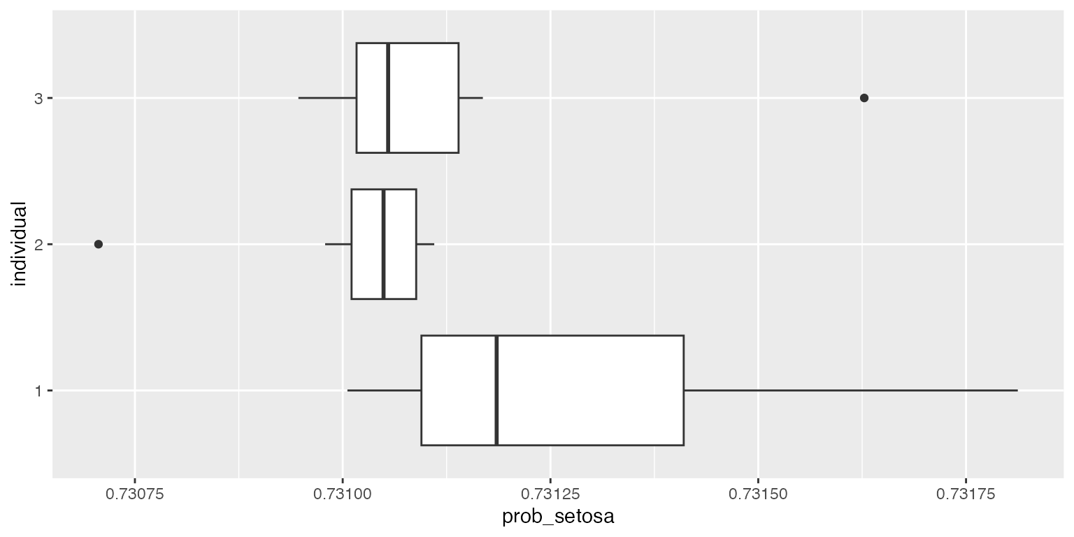
ggplot2::ggplot(df, aes(x=prob_setosa, fill=individual)) + geom_density(alpha=.3)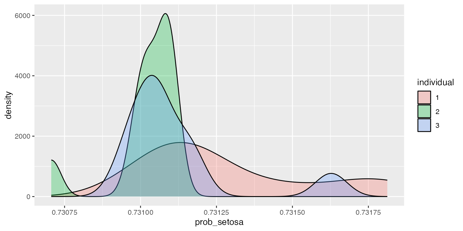
##      Sepal.Length Sepal.Width Petal.Length Petal.Width
## [1,]          5.1         3.5          1.4         0.2
## [2,]          4.6         3.1          1.5         0.2
## [3,]          4.9         3.1          1.5         0.1
## [4,]          5.4         3.7          1.5         0.2
## [5,]          5.2         3.5          1.5         0.2
## [6,]          4.8         3.1          1.6         0.2
obj$summary(X_test, y=y_test,
            class_name = "setosa",
            show_progress=FALSE)
## $Coverage_rate
## [1] 100
##
## $citests
## estimate lower upper p-value signif
## Sepal.Length -0.039134932 -0.06072533 -0.017544534 0.0008803909 ***
## Sepal.Width 0.055710324 0.02112624 0.090294413 0.0026029962 **
## Petal.Length -0.031343320 -0.05821752 -0.004469122 0.0238163346 *
## Petal.Width -0.008896551 -0.06450724 0.046714139 0.7458712257
##
## $signif_codes
## [1] "Signif. codes: 0 ‘***’ 0.001 ‘**’ 0.01 ‘*’ 0.05 ‘.’ 0.1 ‘ ’ 1"
##
## $effects
## ── Data Summary ────────────────────────
## Values
## Name effects
## Number of rows 30
## Number of columns 4
## _______________________
## Column type frequency:
## numeric 4
## ________________________
## Group variables None
##
## ── Variable type: numeric ──────────────────────────────────────────────────────
## skim_variable mean sd p0 p25 p50 p75 p100 hist
## 1 Sepal.Length -0.0391 0.0578 -0.213 -0.0770 -0.0220 0.000655 0.0348 ▁▂▂▃▇
## 2 Sepal.Width 0.0557 0.0926 -0.120 0 0.0219 0.0852 0.324 ▁▇▃▁▁
## 3 Petal.Length -0.0313 0.0720 -0.273 -0.00563 0 0 0.0255 ▁▁▁▁▇
## 4 Petal.Width -0.00890 0.149 -0.292 0 0 0.0175 0.494 ▂▇▃▁▁## Sepal.Length Sepal.Width Petal.Length Petal.Width
## [1,] 5.1 3.5 1.4 0.2
## [2,] 4.6 3.1 1.5 0.2
## [3,] 4.9 3.1 1.5 0.1
## [4,] 5.4 3.7 1.5 0.2
## [5,] 5.2 3.5 1.5 0.2
## [6,] 4.8 3.1 1.6 0.2
obj$summary(X_test, y=y_test,
            class_name = "setosa",
            show_progress=FALSE, type_ci="nonparametric")
## $Coverage_rate
## [1] 100
##
## $citests
## estimate lower upper p-value signif
## Sepal.Length -0.048443334 -0.104589591 -0.00495945 0.05722536 .
## Sepal.Width 0.035202317 -0.002792421 0.08621557 0.12169958
## Petal.Length 0.003582802 -0.035319385 0.02875329 0.82658880
## Petal.Width -0.032667921 -0.127705313 0.04256300 0.45235577
##
## $signif_codes
## [1] "Signif. codes: 0 ‘***’ 0.001 ‘**’ 0.01 ‘*’ 0.05 ‘.’ 0.1 ‘ ’ 1"
##
## $effects
## ── Data Summary ────────────────────────
## Values
## Name effects
## Number of rows 30
## Number of columns 4
## _______________________
## Column type frequency:
## numeric 4
## ________________________
## Group variables None
##
## ── Variable type: numeric ──────────────────────────────────────────────────────
## skim_variable mean sd p0 p25 p50 p75 p100 hist
## 1 Sepal.Length -0.0391 0.0578 -0.213 -0.0770 -0.0220 0.000655 0.0348 ▁▂▂▃▇
## 2 Sepal.Width 0.0557 0.0926 -0.120 0 0.0219 0.0852 0.324 ▁▇▃▁▁
## 3 Petal.Length -0.0313 0.0720 -0.273 -0.00563 0 0 0.0255 ▁▁▁▁▇
## 4 Petal.Width -0.00890 0.149 -0.292 0 0 0.0175 0.494 ▂▇▃▁▁2 - ranger classification
obj <- learningmachine::Classifier$new(method = "ranger",
                                       type_prediction_set="score")
obj$set_level(95)
obj$set_pi_method("bootsplitconformal")
t0 <- proc.time()[3]
obj$fit(X_train, y_train)
cat("Elapsed: ", proc.time()[3] - t0, "s \n")
## Elapsed: 0.115 s
probs <- obj$predict_proba(X_test)
df <- reshape2::melt(probs$sims$setosa[1:3, ])
df$Var2 <- NULL
colnames(df) <- c("individual", "prob_setosa")
df$individual <- as.factor(df$individual)
ggplot2::ggplot(df, aes(x=individual, y=prob_setosa)) + geom_boxplot() + coord_flip()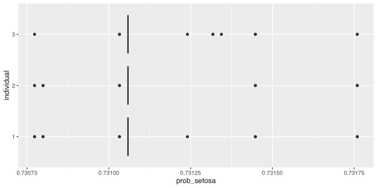
ggplot2::ggplot(df, aes(x=prob_setosa, fill=individual)) + geom_density(alpha=.3)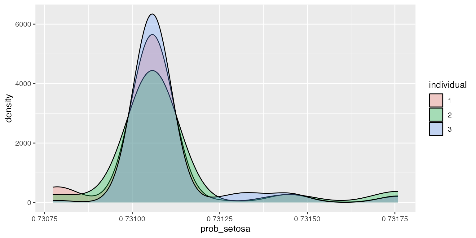
obj$summary(X_test, y=y_test,
            class_name = "setosa",
            show_progress=FALSE)
## $Coverage_rate
## [1] 100
##
## $citests
## estimate lower upper p-value signif
## Sepal.Length -0.039232036 -0.06085041 -0.017613666 0.0008701315 ***
## Sepal.Width 0.055753840 0.02119147 0.090316214 0.0025719853 **
## Petal.Length -0.031600295 -0.05846617 -0.004734417 0.0227458629 *
## Petal.Width -0.008676126 -0.06476250 0.047410244 0.7539793687
##
## $signif_codes
## [1] "Signif. codes: 0 ‘***’ 0.001 ‘**’ 0.01 ‘*’ 0.05 ‘.’ 0.1 ‘ ’ 1"
##
## $effects
## ── Data Summary ────────────────────────
## Values
## Name effects
## Number of rows 30
## Number of columns 4
## _______________________
## Column type frequency:
## numeric 4
## ________________________
## Group variables None
##
## ── Variable type: numeric ──────────────────────────────────────────────────────
## skim_variable mean sd p0 p25 p50 p75 p100 hist
## 1 Sepal.Length -0.0392 0.0579 -0.213 -0.0770 -0.0221 0.000653 0.0343 ▁▂▂▃▇
## 2 Sepal.Width 0.0558 0.0926 -0.119 0 0.0218 0.0854 0.322 ▁▇▃▁▁
## 3 Petal.Length -0.0316 0.0719 -0.270 -0.00566 0 0 0.0257 ▁▁▁▁▇
## 4 Petal.Width -0.00868 0.150 -0.291 0 0 0.0178 0.502 ▂▇▁▁▁
obj$summary(X_test, y=y_test,
            class_index = 2,
            show_progress=FALSE, type_ci="nonparametric")
## $Coverage_rate
## [1] 100
##
## $citests
## estimate lower upper p-value signif
## Sepal.Length 0.005584273 -0.03817798 0.052381504 8.090972e-01
## Sepal.Width -0.136170522 -0.29444020 -0.007446021 6.348879e-02 .
## Petal.Length -0.108256713 -0.51936703 0.208079493 5.599189e-01
## Petal.Width 0.604226657 0.40022576 0.761194883 1.335314e-10 ***
##
## $signif_codes
## [1] "Signif. codes: 0 ‘***’ 0.001 ‘**’ 0.01 ‘*’ 0.05 ‘.’ 0.1 ‘ ’ 1"
##
## $effects
## ── Data Summary ────────────────────────
## Values
## Name effects
## Number of rows 30
## Number of columns 4
## _______________________
## Column type frequency:
## numeric 4
## ________________________
## Group variables None
##
## ── Variable type: numeric ──────────────────────────────────────────────────────
## skim_variable mean sd p0 p25 p50 p75 p100 hist
## 1 Sepal.Length -0.00255 0.0921 -0.242 -0.0216 0 0.0496 0.153 ▁▂▅▇▃
## 2 Sepal.Width -0.0834 0.166 -0.641 -0.125 -0.0409 0.00181 0.170 ▁▁▂▇▃
## 3 Petal.Length -0.436 0.919 -3.27 -0.197 0 0 0.272 ▁▁▁▁▇
## 4 Petal.Width -0.466 1.22 -6.18 -0.295 -0.0597 0 0 ▁▁▁▁▇3 - extratrees classification
obj <- learningmachine::Classifier$new(method = "extratrees",
        pi_method = "bootsplitconformal", type_prediction_set="score")
obj$set_level(95)
t0 <- proc.time()[3]
obj$fit(X_train, y_train)
cat("Elapsed: ", proc.time()[3] - t0, "s \n")
## Elapsed: 0.125 s
probs <- obj$predict_proba(X_test)
df <- reshape2::melt(probs$sims$virginica[1:3, ])
df$Var2 <- NULL
colnames(df) <- c("individual", "prob_virginica")
df$individual <- as.factor(df$individual)
ggplot2::ggplot(df, aes(x=individual, y=prob_virginica)) + geom_boxplot() + coord_flip()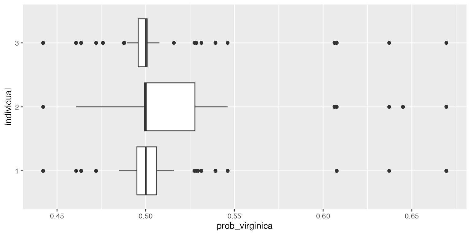
ggplot2::ggplot(df, aes(x=prob_virginica, fill=individual)) + geom_density(alpha=.3)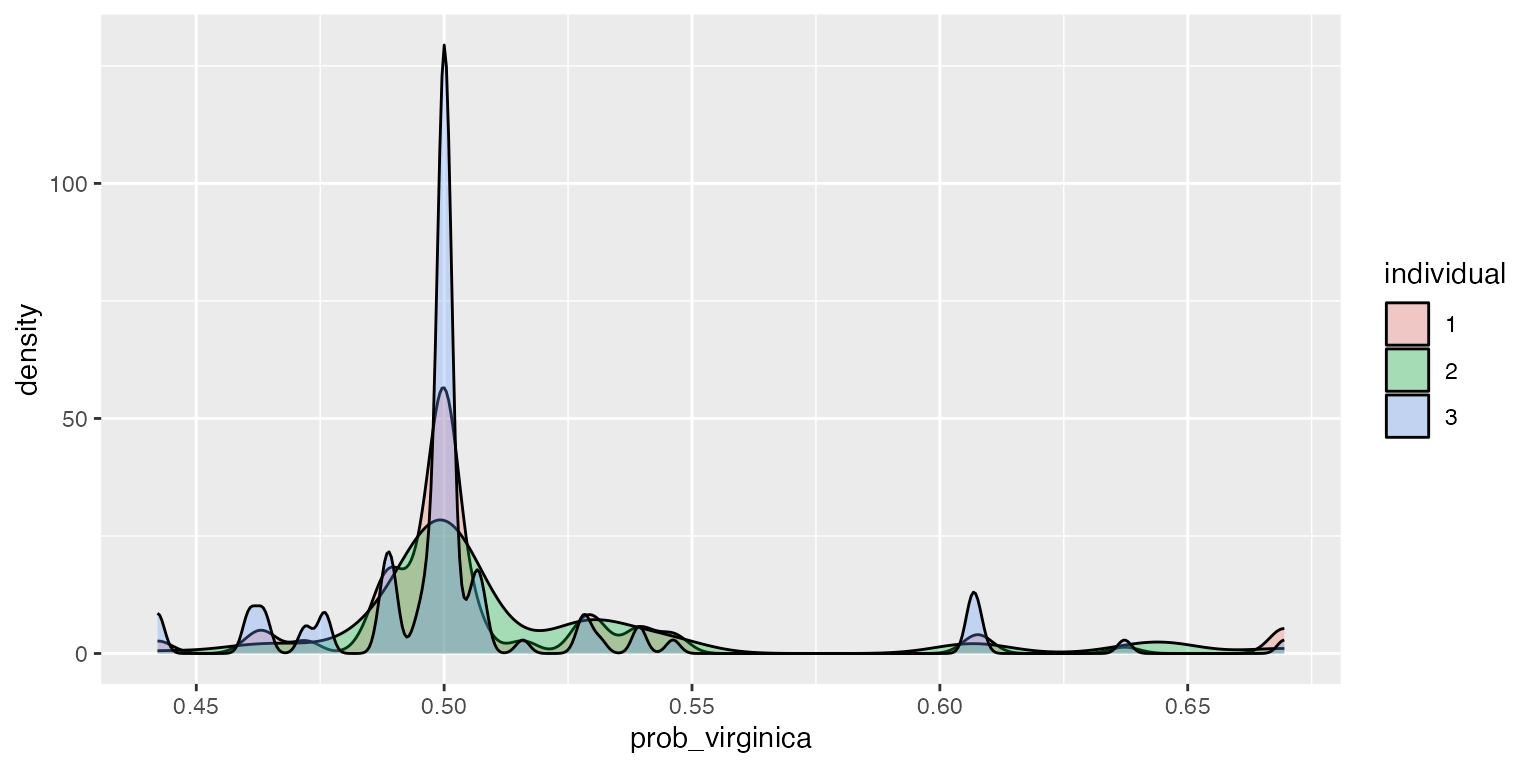
obj$summary(X_test, y=y_test,
            class_name = "virginica",
            show_progress=FALSE)
## $Coverage_rate
## [1] 100
##
## $citests
## estimate lower upper p-value signif
## Sepal.Length 0.036541255 -0.01605960 0.08914210 0.1660389146
## Sepal.Width -0.008665406 -0.08293934 0.06560852 0.8130836281
## Petal.Length 0.367528646 0.17051921 0.56453808 0.0006587430 ***
## Petal.Width 0.657891051 0.31550619 1.00027591 0.0004837876 ***
##
## $signif_codes
## [1] "Signif. codes: 0 ‘***’ 0.001 ‘**’ 0.01 ‘*’ 0.05 ‘.’ 0.1 ‘ ’ 1"
##
## $effects
## ── Data Summary ────────────────────────
## Values
## Name effects
## Number of rows 30
## Number of columns 4
## _______________________
## Column type frequency:
## numeric 4
## ________________________
## Group variables None
##
## ── Variable type: numeric ──────────────────────────────────────────────────────
## skim_variable mean sd p0 p25 p50 p75 p100 hist
## 1 Sepal.Length 0.0365 0.141 -0.247 -0.0246 0.00605 0.0720 0.571 ▁▇▂▁▁
## 2 Sepal.Width -0.00867 0.199 -0.378 -0.0921 -0.0117 0.0154 0.629 ▂▇▁▁▁
## 3 Petal.Length 0.368 0.528 -0.00377 0.00117 0.0920 0.525 1.63 ▇▁▁▁▁
## 4 Petal.Width 0.658 0.917 0 0.0426 0.388 0.678 4.17 ▇▁▁▁▁
obj$summary(X_test, y=y_test,
            class_name = "setosa",
            show_progress=FALSE, type_ci="nonparametric")
## $Coverage_rate
## [1] 100
##
## $citests
## estimate lower upper p-value signif
## Sepal.Length -0.02891381 -0.07856975 0.007642355 1.892264e-01
## Sepal.Width 0.05119133 -0.02477523 0.141328977 2.275907e-01
## Petal.Length 0.00920727 -0.04566300 0.056302475 7.235174e-01
## Petal.Width -0.18756955 -0.25804631 -0.123101638 7.988292e-08 ***
##
## $signif_codes
## [1] "Signif. codes: 0 ‘***’ 0.001 ‘**’ 0.01 ‘*’ 0.05 ‘.’ 0.1 ‘ ’ 1"
##
## $effects
## ── Data Summary ────────────────────────
## Values
## Name effects
## Number of rows 30
## Number of columns 4
## _______________________
## Column type frequency:
## numeric 4
## ________________________
## Group variables None
##
## ── Variable type: numeric ──────────────────────────────────────────────────────
## skim_variable mean sd p0 p25 p50 p75 p100 hist
## 1 Sepal.Length -0.0310 0.0555 -0.171 -0.0616 -0.00914 0.00495 0.0525 ▂▂▃▇▅
## 2 Sepal.Width 0.118 0.161 -0.0922 0.00719 0.0673 0.240 0.565 ▇▇▆▁▂
## 3 Petal.Length -0.0461 0.148 -0.756 -0.0701 0 0.0142 0.0681 ▁▁▁▁▇
## 4 Petal.Width -0.0757 0.271 -1.38 -0.0676 0 0.0273 0.140 ▁▁▁▁▇4 - Penguins dataset
library(palmerpenguins)
data(penguins)
penguins_ <- as.data.frame(palmerpenguins::penguins)

replacement <- median(penguins$bill_length_mm, na.rm = TRUE)
penguins_$bill_length_mm[is.na(penguins$bill_length_mm)] <- replacement

replacement <- median(penguins$bill_depth_mm, na.rm = TRUE)
penguins_$bill_depth_mm[is.na(penguins$bill_depth_mm)] <- replacement

replacement <- median(penguins$flipper_length_mm, na.rm = TRUE)
penguins_$flipper_length_mm[is.na(penguins$flipper_length_mm)] <- replacement

replacement <- median(penguins$body_mass_g, na.rm = TRUE)
penguins_$body_mass_g[is.na(penguins$body_mass_g)] <- replacement

# replacing NA's by the most frequent occurence
penguins_$sex[is.na(penguins$sex)] <- "male" # most frequent

# one-hot encoding for covariates
penguins_mat <- model.matrix(species ~., data=penguins_)[,-1]
penguins_mat <- cbind.data.frame(penguins_$species, penguins_mat)
penguins_mat <- as.data.frame(penguins_mat)
colnames(penguins_mat)[1] <- "species"

y <- penguins_mat$species
X <- as.matrix(penguins_mat[,2:ncol(penguins_mat)])

n <- nrow(X)
p <- ncol(X)

set.seed(1234)
index_train <- sample(1:n, size=floor(0.8*n))
X_train <- X[index_train, ]
y_train <- factor(y[index_train])
X_test <- X[-index_train, ][1:5, ]
y_test <- factor(y[-index_train][1:5])
obj <- learningmachine::Classifier$new(method = "extratrees",
                                       type_prediction_set="score")
obj$set_pi_method("bootsplitconformal")
obj$set_level(95)
obj$set_B(10L)
t0 <- proc.time()[3]
obj$fit(X_train, y_train)
cat("Elapsed: ", proc.time()[3] - t0, "s \n")
## Elapsed: 0.243 s
probs <- obj$predict_proba(X_test)
df <- reshape2::melt(probs$sims[[1]][1:3, ])
df$Var2 <- NULL
colnames(df) <- c("individual", "prob_Adelie")
df$individual <- as.factor(df$individual)
ggplot2::ggplot(df, aes(x=individual, y=prob_Adelie)) + geom_boxplot() + coord_flip()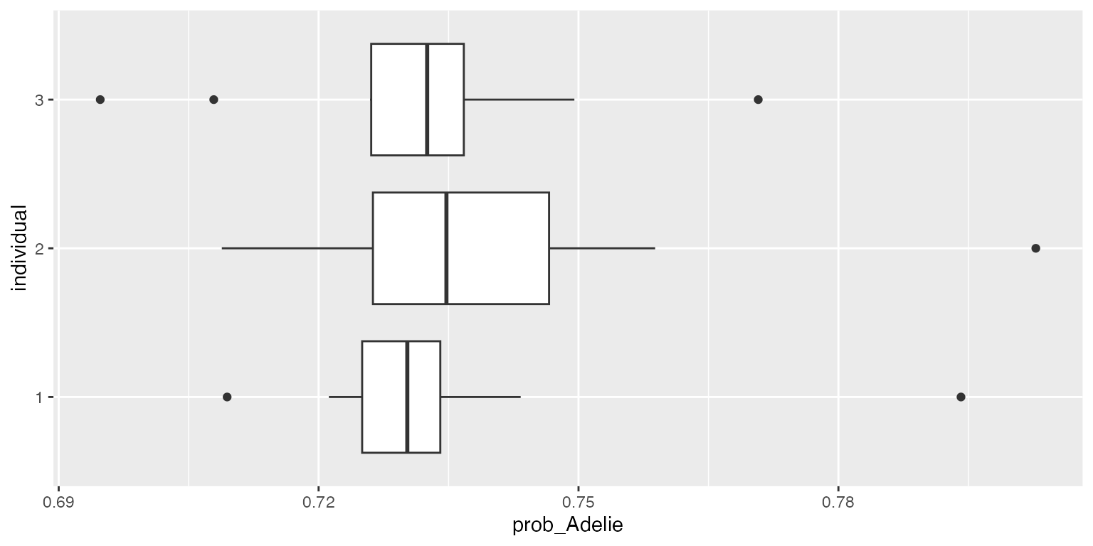
ggplot2::ggplot(df, aes(x=prob_Adelie, fill=individual)) + geom_density(alpha=.3)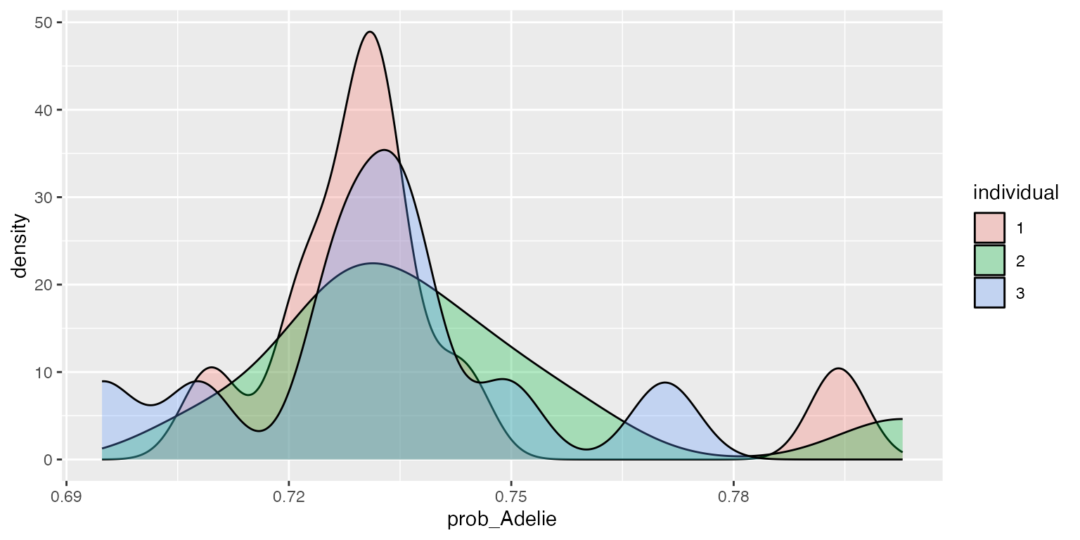
obj$summary(X_test, y=y_test,
            class_name = "Adelie",
            show_progress=FALSE)
## $Coverage_rate
## [1] 100
##
## $citests
## estimate lower upper p-value signif
## islandDream 0.000000e+00 NaN NaN NaN
## islandTorgersen -1.778468e-02 -3.459725e-02 -9.721090e-04 0.04251686 *
## bill_length_mm 5.776485e-03 -5.537377e-03 1.709035e-02 0.22929028
## bill_depth_mm 3.407051e-03 -1.958522e-03 8.772623e-03 0.15268182
## flipper_length_mm -4.827102e-04 -1.785223e-03 8.198026e-04 0.36165192
## body_mass_g -2.325034e-05 -5.796378e-05 1.146310e-05 0.13646280
## sexmale -7.978043e-03 -2.213090e-02 6.174818e-03 0.19261298
## year -3.352928e-05 -8.057931e-05 1.352074e-05 0.11899484
##
## $signif_codes
## [1] "Signif. codes: 0 ‘***’ 0.001 ‘**’ 0.01 ‘*’ 0.05 ‘.’ 0.1 ‘ ’ 1"
##
## $effects
## ── Data Summary ────────────────────────
## Values
## Name effects
## Number of rows 5
## Number of columns 8
## _______________________
## Column type frequency:
## numeric 8
## ________________________
## Group variables None
##
## ── Variable type: numeric ──────────────────────────────────────────────────────
## skim_variable mean sd p0 p25 p50
## 1 islandDream 0 0 0 0 0
## 2 islandTorgersen -0.0178 0.0135 -0.0344 -0.0270 -0.0190
## 3 bill_length_mm 0.00578 0.00911 0.000434 0.00100 0.00263
## 4 bill_depth_mm 0.00341 0.00432 -0.00118 0.00175 0.00275
## 5 flipper_length_mm -0.000483 0.00105 -0.00233 -0.000239 -0.0000659
## 6 body_mass_g -0.0000233 0.0000280 -0.0000606 -0.0000442 -0.00000943
## 7 sexmale -0.00798 0.0114 -0.0223 -0.0184 0
## 8 year -0.0000335 0.0000379 -0.0000969 -0.0000349 -0.0000213
## p75 p100 hist
## 1 0 0 ▁▁▇▁▁
## 2 -0.00591 -0.00263 ▃▃▃▁▇
## 3 0.00284 0.0220 ▇▁▁▁▂
## 4 0.00320 0.0105 ▂▇▁▁▂
## 5 -0.0000350 0.000258 ▂▁▁▁▇
## 6 -0.00000863 0.00000657 ▃▃▁▇▃
## 7 0 0.000842 ▅▁▁▁▇
## 8 -0.0000173 0.00000271 ▂▁▁▇▂rvfl
obj <- learningmachine::Classifier$new(method = "rvfl",
                                type_prediction_set="score")
obj$set_pi_method("bootsplitconformal")
obj$set_level(95)
obj$set_B(10L)
t0 <- proc.time()[3]
obj$fit(X_train, y_train)
cat("Elapsed: ", proc.time()[3] - t0, "s \n")
## Elapsed: 0.066 s
probs <- obj$predict_proba(X_test)
df <- reshape2::melt(probs$sims[[1]][1:3, ])
df$Var2 <- NULL
colnames(df) <- c("individual", "prob_Adelie")
df$individual <- as.factor(df$individual)
ggplot2::ggplot(df, aes(x=individual, y=prob_Adelie)) + geom_boxplot() + coord_flip()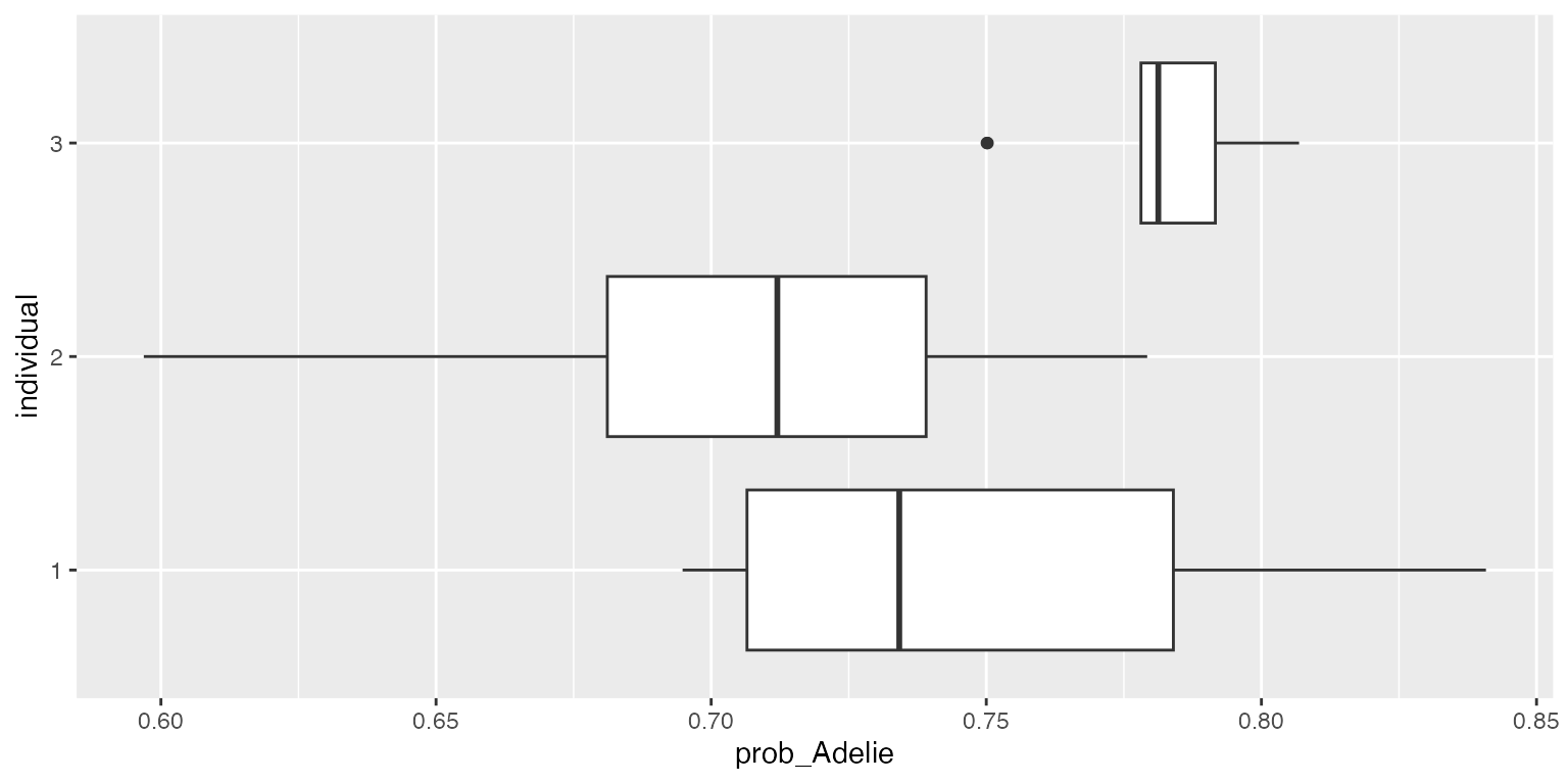
ggplot2::ggplot(df, aes(x=prob_Adelie, fill=individual)) + geom_density(alpha=.3)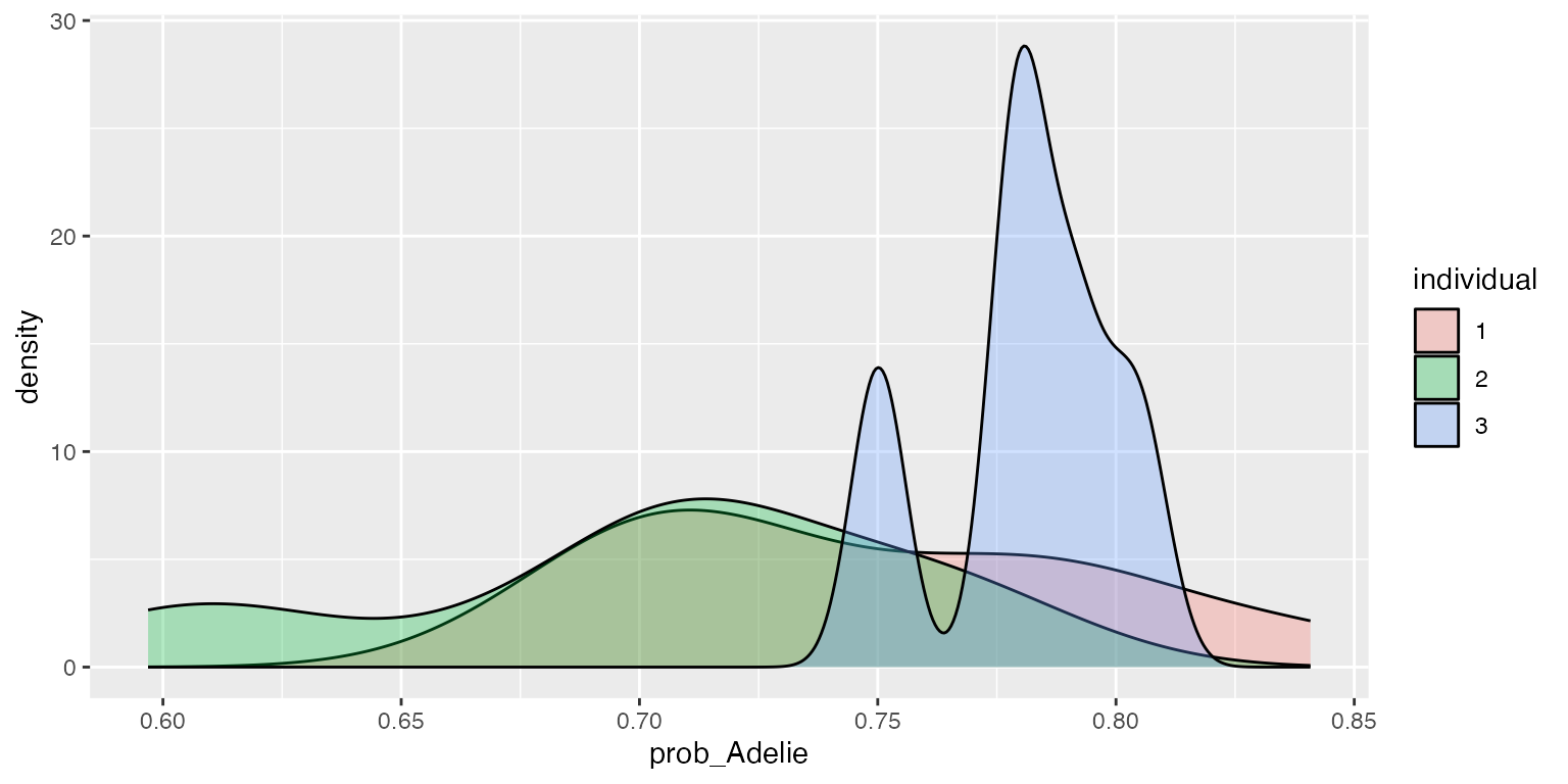
obj$summary(X_test, y=y_test,
            class_name = "Adelie",
            show_progress=FALSE)
## $Coverage_rate
## [1] 100
##
## $citests
## estimate lower upper p-value signif
## islandDream 0.4802248563 0.4780044748 0.4824452379 4.614437e-11 ***
## islandTorgersen -0.2959594072 -0.3063930678 -0.2855257465 1.557925e-07 ***
## bill_length_mm 0.2003956489 0.1963455026 0.2044457951 1.684113e-08 ***
## bill_depth_mm 0.0508209573 0.0479212470 0.0537206676 1.067137e-06 ***
## flipper_length_mm -0.0224653400 -0.0227350465 -0.0221956335 2.097271e-09 ***
## body_mass_g -0.0001692677 -0.0001723101 -0.0001662252 1.053542e-08 ***
## sexmale -0.4310257052 -0.4393042529 -0.4227471575 1.373600e-08 ***
## year -0.0102992883 -0.0110718998 -0.0095266769 3.181998e-06 ***
##
## $signif_codes
## [1] "Signif. codes: 0 ‘***’ 0.001 ‘**’ 0.01 ‘*’ 0.05 ‘.’ 0.1 ‘ ’ 1"
##
## $effects
## ── Data Summary ────────────────────────
## Values
## Name effects
## Number of rows 5
## Number of columns 8
## _______________________
## Column type frequency:
## numeric 8
## ________________________
## Group variables None
##
## ── Variable type: numeric ──────────────────────────────────────────────────────
## skim_variable mean sd p0 p25 p50 p75
## 1 islandDream 0.480 0.00179 0.478 0.479 0.481 0.482
## 2 islandTorgersen -0.296 0.00840 -0.311 -0.294 -0.293 -0.292
## 3 bill_length_mm 0.200 0.00326 0.198 0.199 0.200 0.200
## 4 bill_depth_mm 0.0508 0.00234 0.0467 0.0512 0.0516 0.0521
## 5 flipper_length_mm -0.0225 0.000217 -0.0226 -0.0226 -0.0226 -0.0224
## 6 body_mass_g -0.000169 0.00000245 -0.000173 -0.000169 -0.000169 -0.000168
## 7 sexmale -0.431 0.00667 -0.442 -0.430 -0.429 -0.427
## 8 year -0.0103 0.000622 -0.0112 -0.0105 -0.0102 -0.00980
## p100 hist
## 1 0.482 ▂▂▁▁▇
## 2 -0.289 ▂▁▁▂▇
## 3 0.206 ▇▇▁▁▃
## 4 0.0524 ▂▁▁▂▇
## 5 -0.0221 ▇▁▂▁▂
## 6 -0.000167 ▃▁▁▇▇
## 7 -0.426 ▃▁▁▇▇
## 8 -0.00972 ▃▁▃▃▇