Correlation tests for the shocks (if Gaussian copula)

This function performs correlation tests for the shocks generated by simshocks.

esgcortest(
  x,
  alternative = c("two.sided", "less", "greater"),
  method = c("pearson", "kendall", "spearman"),
  conf.level = 0.95
)

Arguments

x: gaussian (bivariate) shocks, with correlation, generated by simshocks (if Gaussian copula).
alternative: indicates the alternative hypothesis and must be one of "two.sided", "greater" or "less".
method: which correlation coefficient is to be used for the test : "pearson", "kendall", or "spearman".
conf.level: confidence level.

Value

a list with 2 components : estimated correlation coefficients, and confidence intervals for the estimated correlations.

References

D. J. Best & D. E. Roberts (1975), Algorithm AS 89: The Upper Tail Probabilities of Spearman's rho. Applied Statistics, 24, 377-379.

Myles Hollander & Douglas A. Wolfe (1973), Nonparametric Statistical Methods. New York: John Wiley & Sons. Pages 185-194 (Kendall and Spearman tests).

Author

T. Moudiki + stats package

Examples


nb <- 500

s0.par1 <- simshocks(n = nb, horizon = 3, frequency = "semi",
family = 1, par = 0.2)

s0.par2 <- simshocks(n = nb, horizon = 3, frequency = "semi", 
family = 1, par = 0.8)

(test1 <- esgcortest(s0.par1))
#> $cor.estimate
#> Time Series:
#> Start = c(0, 2) 
#> End = c(3, 1) 
#> Frequency = 2 
#> [1] 0.17019209 0.09279227 0.18718789 0.22185835 0.14601034 0.19899949
#> 
#> $conf.int
#> Time Series:
#> Start = c(0, 2) 
#> End = c(3, 1) 
#> Frequency = 2 
#>        Series 1  Series 2
#> 0.5 0.083751429 0.2540906
#> 1.0 0.005143531 0.1790261
#> 1.5 0.101157771 0.2704393
#> 2.0 0.136829774 0.3036416
#> 2.5 0.059076143 0.2307465
#> 3.0 0.113285783 0.2817730
#> 
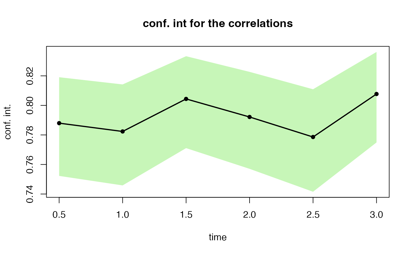
(test2 <- esgcortest(s0.par2))
#> $cor.estimate
#> Time Series:
#> Start = c(0, 2) 
#> End = c(3, 1) 
#> Frequency = 2 
#> [1] 0.7879729 0.7823533 0.8043743 0.7921554 0.7786005 0.8077114
#> 
#> $conf.int
#> Time Series:
#> Start = c(0, 2) 
#> End = c(3, 1) 
#> Frequency = 2 
#>      Series 1  Series 2
#> 0.5 0.7522620 0.8190677
#> 1.0 0.7458304 0.8141866
#> 1.5 0.7710721 0.8332881
#> 2.0 0.7570532 0.8226977
#> 2.5 0.7415392 0.8109245
#> 3.0 0.7749064 0.8361767
#> 
#par(mfrow=c(2, 1))
esgplotbands(test1)

esgplotbands(test2)