This function plots colored bands for time series percentiles and confidence
intervals. You can use it for outputs from simdiff,
esgmartingaletest, esgcortest.
esgplotbands(x, ...)Arguments
- x
a times series object
- ...
additionnal (optional) parameters provided to
plot
See also
Examples
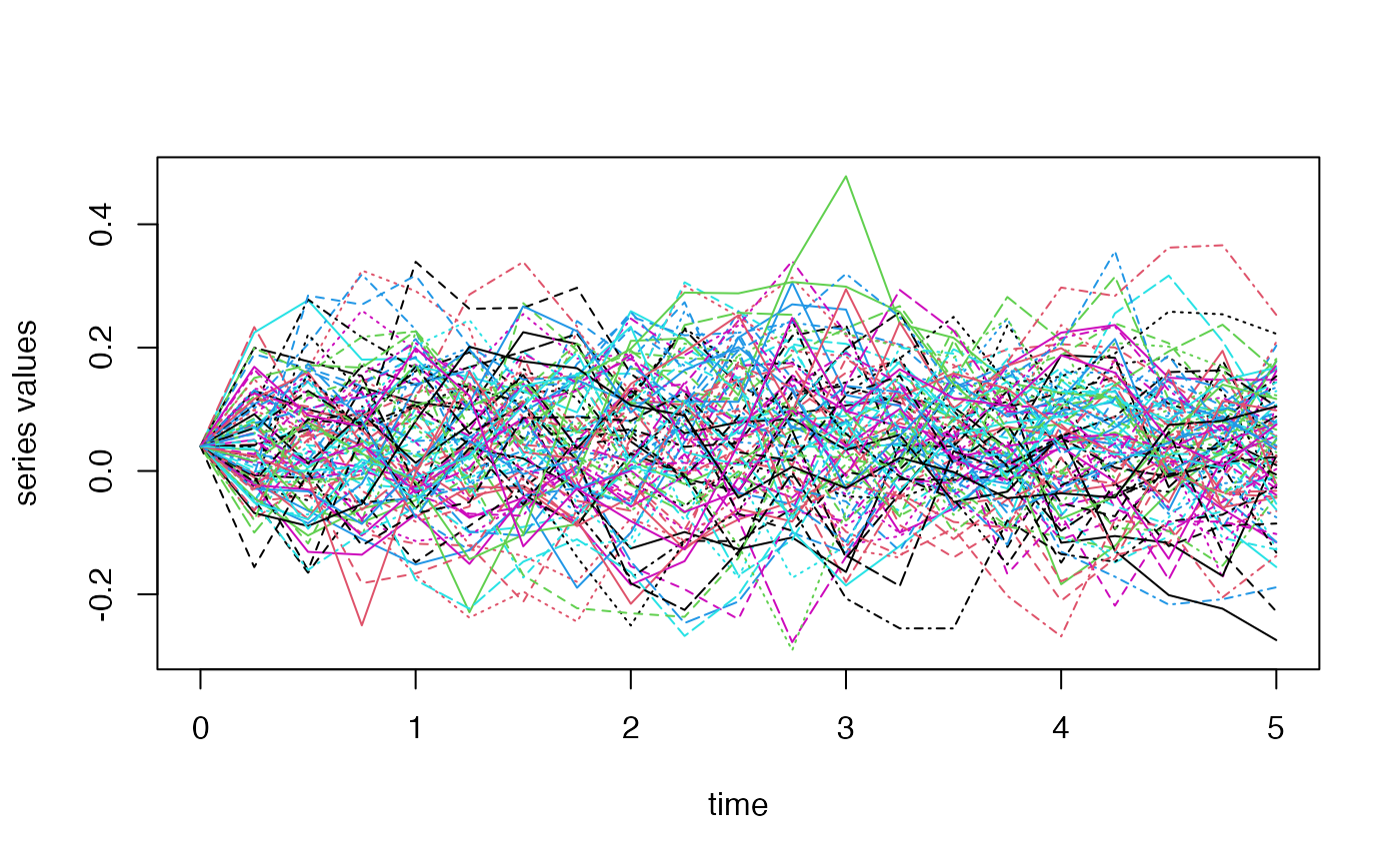
# Times series
kappa <- 1.5
V0 <- theta <- 0.04
sigma <- 0.2
theta1 <- kappa*theta
theta2 <- kappa
theta3 <- sigma
x <- simdiff(n = 100, horizon = 5,
frequency = "quart",
model = "OU",
x0 = V0, theta1 = theta1, theta2 = theta2, theta3 = theta3)
#par(mfrow=c(2,1))
esgplotbands(x, xlab = "time", ylab = "values")
 matplot(as.vector(time(x)), x, type = 'l', xlab = "time", ylab = "series values")
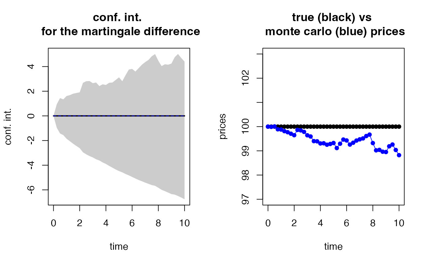
 # Martingale test
r0 <- 0.03
S0 <- 100
sigma0 <- 0.1
nbScenarios <- 100
horizon0 <- 10
eps0 <- simshocks(n = nbScenarios, horizon = horizon0, frequency = "quart",
method = "anti")
sim.GBM <- simdiff(n = nbScenarios, horizon = horizon0, frequency = "quart",
model = "GBM",
x0 = S0, theta1 = r0, theta2 = sigma0,
eps = eps0)
mc.test <- esgmartingaletest(r = r0, X = sim.GBM, p0 = S0, alpha = 0.05)
#>
#> martingale '1=1' one Sample t-test
#>
#> alternative hypothesis: true mean of the martingale difference is not equal to 0
#>
#> df = 99
#> t p-value
#> 0 Q2 -1.5893012 0.1151810
#> 0 Q3 -1.0308985 0.3051004
#> 0 Q4 -1.1816807 0.2401632
#> 1 Q1 -0.9994328 0.3200217
#> 1 Q2 -0.9975481 0.3209305
#> 1 Q3 -0.9616265 0.3385801
#> 1 Q4 -0.9648799 0.3369560
#> 2 Q1 -0.9697852 0.3345169
#> 2 Q2 -0.6268720 0.5321861
#> 2 Q3 -0.6069495 0.5452739
#> 2 Q4 -0.6321323 0.5287576
#> 3 Q1 -0.7319134 0.4659505
#> 3 Q2 -0.7397776 0.4611856
#> 3 Q3 -0.8892875 0.3760044
#> 3 Q4 -0.8520924 0.3962194
#> 4 Q1 -0.8972630 0.3717554
#> 4 Q2 -0.8478169 0.3985851
#> 4 Q3 -0.8617621 0.3909010
#> 4 Q4 -0.8027883 0.4240202
#> 5 Q1 -0.7461950 0.4573179
#> 5 Q2 -0.8797694 0.3811148
#> 5 Q3 -0.7223612 0.4717754
#> 5 Q4 -0.5950943 0.5531383
#> 6 Q1 -0.5996844 0.5500866
#> 6 Q2 -0.6835096 0.4958815
#> 6 Q3 -0.6201930 0.5365557
#> 6 Q4 -0.5575577 0.5784050
#> 7 Q1 -0.5188512 0.6050224
#> 7 Q2 -0.4895547 0.6255320
#> 7 Q3 -0.4335887 0.6655305
#> 7 Q4 -0.4019780 0.6885668
#> 8 Q1 -0.5517836 0.5823401
#> 8 Q2 -0.6854329 0.4946727
#> 8 Q3 -0.6607812 0.5102873
#> 8 Q4 -0.6841250 0.4954946
#> 9 Q1 -0.6756343 0.5008480
#> 9 Q2 -0.5573952 0.5785155
#> 9 Q3 -0.5141757 0.6082750
#> 9 Q4 -0.6023588 0.5483125
#> 10 Q1 -0.6864080 0.4940604
#>
#> 95 percent confidence intervals for the mean :
#> c.i lower bound c.i upper bound
#> 0 Q1 0.000000 0.0000000
#> 0 Q2 -1.704155 0.1883292
#> 0 Q3 -2.162324 0.6836831
#> 0 Q4 -2.296103 0.5820486
#> 1 Q1 -2.590482 0.8550150
#> 1 Q2 -2.786158 0.9219423
#> 1 Q3 -2.989586 1.0377748
#> 1 Q4 -3.170991 1.0960333
#> 2 Q1 -3.346892 1.1493536
#> 2 Q2 -3.678659 1.9123091
#> 2 Q3 -3.843892 2.0431211
#> 2 Q4 -3.981028 2.0573271
#> 3 Q1 -4.090321 1.8858902
#> 3 Q2 -4.240255 1.9371331
#> 3 Q3 -4.336025 1.6522132
#> 3 Q4 -4.493488 1.7935944
#> 4 Q1 -4.615875 1.7412037
#> 4 Q2 -4.776183 1.9165219
#> 4 Q3 -4.916665 1.9391341
#> 4 Q4 -5.063956 2.1466419
#> 5 Q1 -5.190505 2.3534762
#> 5 Q2 -5.292663 2.0410253
#> 5 Q3 -5.425924 2.5296641
#> 5 Q4 -5.536569 2.9817938
#> 6 Q1 -5.662485 3.0341306
#> 6 Q2 -5.788609 2.8223605
#> 6 Q3 -5.908501 3.0944961
#> 6 Q4 -6.012426 3.3746828
#> 7 Q1 -6.120358 3.5830279
#> 7 Q2 -6.218107 3.7570037
#> 7 Q3 -6.317987 4.0519588
#> 7 Q4 -6.374286 4.2266636
#> 8 Q1 -6.533080 3.6901422
#> 8 Q2 -6.697632 3.2583963
#> 8 Q3 -6.808017 3.4064195
#> 8 Q4 -6.922402 3.3727911
#> 9 Q1 -7.041456 3.4642265
#> 9 Q2 -7.084925 3.9773675
#> 9 Q3 -7.196704 4.2345033
#> 9 Q4 -7.319541 3.9104080
#> 10 Q1 -7.459425 3.6249599
esgplotbands(mc.test)
# Martingale test
r0 <- 0.03
S0 <- 100
sigma0 <- 0.1
nbScenarios <- 100
horizon0 <- 10
eps0 <- simshocks(n = nbScenarios, horizon = horizon0, frequency = "quart",
method = "anti")
sim.GBM <- simdiff(n = nbScenarios, horizon = horizon0, frequency = "quart",
model = "GBM",
x0 = S0, theta1 = r0, theta2 = sigma0,
eps = eps0)
mc.test <- esgmartingaletest(r = r0, X = sim.GBM, p0 = S0, alpha = 0.05)
#>
#> martingale '1=1' one Sample t-test
#>
#> alternative hypothesis: true mean of the martingale difference is not equal to 0
#>
#> df = 99
#> t p-value
#> 0 Q2 -1.5893012 0.1151810
#> 0 Q3 -1.0308985 0.3051004
#> 0 Q4 -1.1816807 0.2401632
#> 1 Q1 -0.9994328 0.3200217
#> 1 Q2 -0.9975481 0.3209305
#> 1 Q3 -0.9616265 0.3385801
#> 1 Q4 -0.9648799 0.3369560
#> 2 Q1 -0.9697852 0.3345169
#> 2 Q2 -0.6268720 0.5321861
#> 2 Q3 -0.6069495 0.5452739
#> 2 Q4 -0.6321323 0.5287576
#> 3 Q1 -0.7319134 0.4659505
#> 3 Q2 -0.7397776 0.4611856
#> 3 Q3 -0.8892875 0.3760044
#> 3 Q4 -0.8520924 0.3962194
#> 4 Q1 -0.8972630 0.3717554
#> 4 Q2 -0.8478169 0.3985851
#> 4 Q3 -0.8617621 0.3909010
#> 4 Q4 -0.8027883 0.4240202
#> 5 Q1 -0.7461950 0.4573179
#> 5 Q2 -0.8797694 0.3811148
#> 5 Q3 -0.7223612 0.4717754
#> 5 Q4 -0.5950943 0.5531383
#> 6 Q1 -0.5996844 0.5500866
#> 6 Q2 -0.6835096 0.4958815
#> 6 Q3 -0.6201930 0.5365557
#> 6 Q4 -0.5575577 0.5784050
#> 7 Q1 -0.5188512 0.6050224
#> 7 Q2 -0.4895547 0.6255320
#> 7 Q3 -0.4335887 0.6655305
#> 7 Q4 -0.4019780 0.6885668
#> 8 Q1 -0.5517836 0.5823401
#> 8 Q2 -0.6854329 0.4946727
#> 8 Q3 -0.6607812 0.5102873
#> 8 Q4 -0.6841250 0.4954946
#> 9 Q1 -0.6756343 0.5008480
#> 9 Q2 -0.5573952 0.5785155
#> 9 Q3 -0.5141757 0.6082750
#> 9 Q4 -0.6023588 0.5483125
#> 10 Q1 -0.6864080 0.4940604
#>
#> 95 percent confidence intervals for the mean :
#> c.i lower bound c.i upper bound
#> 0 Q1 0.000000 0.0000000
#> 0 Q2 -1.704155 0.1883292
#> 0 Q3 -2.162324 0.6836831
#> 0 Q4 -2.296103 0.5820486
#> 1 Q1 -2.590482 0.8550150
#> 1 Q2 -2.786158 0.9219423
#> 1 Q3 -2.989586 1.0377748
#> 1 Q4 -3.170991 1.0960333
#> 2 Q1 -3.346892 1.1493536
#> 2 Q2 -3.678659 1.9123091
#> 2 Q3 -3.843892 2.0431211
#> 2 Q4 -3.981028 2.0573271
#> 3 Q1 -4.090321 1.8858902
#> 3 Q2 -4.240255 1.9371331
#> 3 Q3 -4.336025 1.6522132
#> 3 Q4 -4.493488 1.7935944
#> 4 Q1 -4.615875 1.7412037
#> 4 Q2 -4.776183 1.9165219
#> 4 Q3 -4.916665 1.9391341
#> 4 Q4 -5.063956 2.1466419
#> 5 Q1 -5.190505 2.3534762
#> 5 Q2 -5.292663 2.0410253
#> 5 Q3 -5.425924 2.5296641
#> 5 Q4 -5.536569 2.9817938
#> 6 Q1 -5.662485 3.0341306
#> 6 Q2 -5.788609 2.8223605
#> 6 Q3 -5.908501 3.0944961
#> 6 Q4 -6.012426 3.3746828
#> 7 Q1 -6.120358 3.5830279
#> 7 Q2 -6.218107 3.7570037
#> 7 Q3 -6.317987 4.0519588
#> 7 Q4 -6.374286 4.2266636
#> 8 Q1 -6.533080 3.6901422
#> 8 Q2 -6.697632 3.2583963
#> 8 Q3 -6.808017 3.4064195
#> 8 Q4 -6.922402 3.3727911
#> 9 Q1 -7.041456 3.4642265
#> 9 Q2 -7.084925 3.9773675
#> 9 Q3 -7.196704 4.2345033
#> 9 Q4 -7.319541 3.9104080
#> 10 Q1 -7.459425 3.6249599
esgplotbands(mc.test)
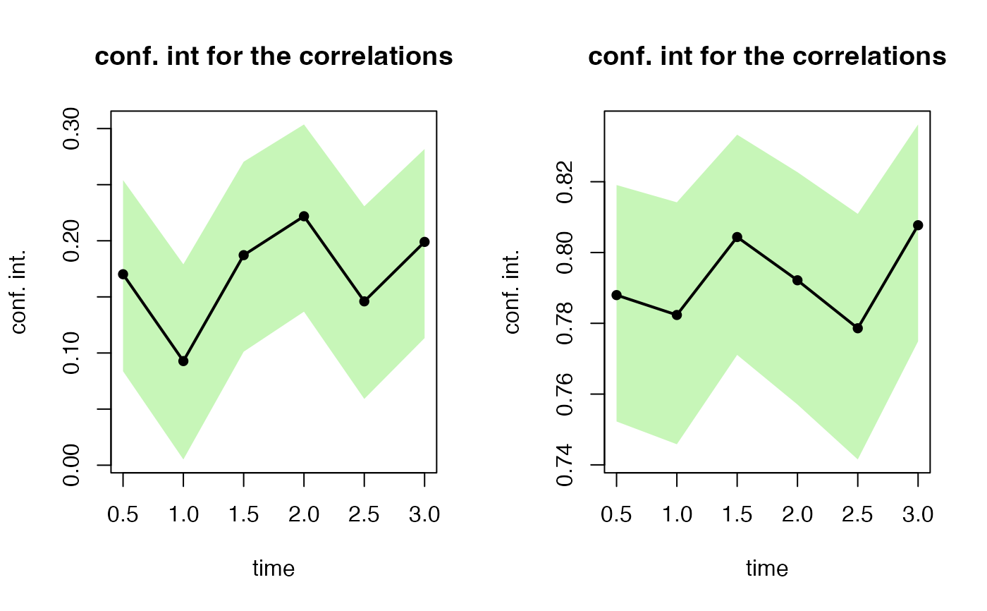
 # Correlation test
nb <- 500
s0.par1 <- simshocks(n = nb, horizon = 3, frequency = "semi",
family = 1, par = 0.2)
s0.par2 <- simshocks(n = nb, horizon = 3, frequency = "semi",
family = 1, par = 0.8)
(test1 <- esgcortest(s0.par1))
#> $cor.estimate
#> Time Series:
#> Start = c(0, 2)
#> End = c(3, 1)
#> Frequency = 2
#> [1] 0.17019209 0.09279227 0.18718789 0.22185835 0.14601034 0.19899949
#>
#> $conf.int
#> Time Series:
#> Start = c(0, 2)
#> End = c(3, 1)
#> Frequency = 2
#> Series 1 Series 2
#> 0.5 0.083751429 0.2540906
#> 1.0 0.005143531 0.1790261
#> 1.5 0.101157771 0.2704393
#> 2.0 0.136829774 0.3036416
#> 2.5 0.059076143 0.2307465
#> 3.0 0.113285783 0.2817730
#>
(test2 <- esgcortest(s0.par2))
#> $cor.estimate
#> Time Series:
#> Start = c(0, 2)
#> End = c(3, 1)
#> Frequency = 2
#> [1] 0.7879729 0.7823533 0.8043743 0.7921554 0.7786005 0.8077114
#>
#> $conf.int
#> Time Series:
#> Start = c(0, 2)
#> End = c(3, 1)
#> Frequency = 2
#> Series 1 Series 2
#> 0.5 0.7522620 0.8190677
#> 1.0 0.7458304 0.8141866
#> 1.5 0.7710721 0.8332881
#> 2.0 0.7570532 0.8226977
#> 2.5 0.7415392 0.8109245
#> 3.0 0.7749064 0.8361767
#>
#par(mfrow=c(2, 1))
esgplotbands(test1)
esgplotbands(test2)
# Correlation test
nb <- 500
s0.par1 <- simshocks(n = nb, horizon = 3, frequency = "semi",
family = 1, par = 0.2)
s0.par2 <- simshocks(n = nb, horizon = 3, frequency = "semi",
family = 1, par = 0.8)
(test1 <- esgcortest(s0.par1))
#> $cor.estimate
#> Time Series:
#> Start = c(0, 2)
#> End = c(3, 1)
#> Frequency = 2
#> [1] 0.17019209 0.09279227 0.18718789 0.22185835 0.14601034 0.19899949
#>
#> $conf.int
#> Time Series:
#> Start = c(0, 2)
#> End = c(3, 1)
#> Frequency = 2
#> Series 1 Series 2
#> 0.5 0.083751429 0.2540906
#> 1.0 0.005143531 0.1790261
#> 1.5 0.101157771 0.2704393
#> 2.0 0.136829774 0.3036416
#> 2.5 0.059076143 0.2307465
#> 3.0 0.113285783 0.2817730
#>
(test2 <- esgcortest(s0.par2))
#> $cor.estimate
#> Time Series:
#> Start = c(0, 2)
#> End = c(3, 1)
#> Frequency = 2
#> [1] 0.7879729 0.7823533 0.8043743 0.7921554 0.7786005 0.8077114
#>
#> $conf.int
#> Time Series:
#> Start = c(0, 2)
#> End = c(3, 1)
#> Frequency = 2
#> Series 1 Series 2
#> 0.5 0.7522620 0.8190677
#> 1.0 0.7458304 0.8141866
#> 1.5 0.7710721 0.8332881
#> 2.0 0.7570532 0.8226977
#> 2.5 0.7415392 0.8109245
#> 3.0 0.7749064 0.8361767
#>
#par(mfrow=c(2, 1))
esgplotbands(test1)
esgplotbands(test2)