Simulation of diffusion processes.

This function makes simulations of diffusion processes, that are building blocks for various risk factors' models.

simdiff(
  n,
  horizon,
  frequency = c("annual", "semi-annual", "quarterly", "monthly", "weekly", "daily"),
  model = c("GBM", "CIR", "OU"),
  x0,
  theta1 = NULL,
  theta2 = NULL,
  theta3 = NULL,
  lambda = NULL,
  mu_z = NULL,
  sigma_z = NULL,
  p = NULL,
  eta_up = NULL,
  eta_down = NULL,
  eps = NULL,
  start = NULL,
  seed = 123
)

Arguments

n

number of independent observations.

horizon

horizon of projection.

frequency

either "annual", "semi-annual", "quarterly", "monthly", "weekly", or "daily" (1, 1/2, 1/4, 1/12, 1/52, 1/252).

model

either Geometric Brownian motion-like ("GBM"), Cox-Ingersoll-Ross ("CIR"), or Ornstein-Uhlenbeck ("OU").

GBM-like (GBM, Merton, Kou, Heston, Bates)

$$dX_t = \theta_1(t) X_t dt + \theta_2(t) X_t dW_t + X_t JdN_t$$

CIR

$$dX_t = (\theta_1 - \theta_2 X_t) dt + \theta_3\sqrt(X_t) dW_t$$

Ornstein-Uhlenbeck $$dX_t = (\theta_1 - \theta_2 X_t)dt + \theta_3 dW_t$$

Where $(W_t)_t$ is a standard brownian motion :

$$dW_t ~~ \epsilon \sqrt(dt)$$

and $$\epsilon ~~ N(0, 1)$$

The $\epsilon$ is a gaussian increment that can be an output from simshocks.

For 'GBM-like', $\theta_1$ and $\theta_2$ can be held constant, and the jumps part $JdN_t$ is optional. In case the jumps are used, they arise following a Poisson process $(N_t)$, with intensities $J$ drawn either from lognormal or asymmetric double-exponential distribution.

x0

starting value of the process.

theta1

a numeric for model = "GBM", model = "CIR", model = "OU". Can also be a time series object (an output from simdiff with the same number of scenarios, horizon and frequency) for model = "GBM", and time-varying parameters.

theta2

theta3

a numeric, volatility for model = "CIR" and model = "OU".

lambda

intensity of the Poisson process counting the jumps. Optional.

mu_z

mean parameter for the lognormal jumps size. Optional.

sigma_z

standard deviation parameter for the lognormal jumps size. Optional.

p

probability of positive jumps. Must belong to ]0, 1[. Optional.

eta_up

mean of positive jumps in Kou's model. Must belong to ]0, 1[. Optional.

eta_down

mean of negative jumps. Must belong to ]0, 1[. Optional.

eps

gaussian shocks. If not provided, independent shocks are generated internally by the function. Otherwise, for custom shocks, must be an output from simshocks.

start

the time of the first observation. Either a single number or a vector of two numbers (the second of which is an integer), which specify a natural time unit and a (1-based) number of samples into the time unit. See `?ts`.

seed

reproducibility seed

Value

a time series object.

References

Black, F., Scholes, M.S. (1973) The pricing of options and corporate liabilities, Journal of Political Economy, 81, 637-654.

Cox, J.C., Ingersoll, J.E., Ross, S.A. (1985) A theory of the term structure of interest rates, Econometrica, 53, 385-408.

Iacus, S. M. (2009). Simulation and inference for stochastic differential equations: with R examples (Vol. 1). Springer.

Glasserman, P. (2004). Monte Carlo methods in financial engineering (Vol. 53). Springer.

Kou S, (2002), A jump diffusion model for option pricing, Management Sci- ence Vol. 48, 1086-1101.

Merton, R. C. (1976). Option pricing when underlying stock returns are discontinuous. Journal of financial economics, 3(1), 125-144.

Uhlenbeck, G. E., Ornstein, L. S. (1930) On the theory of Brownian motion, Phys. Rev., 36, 823-841.

Vasicek, O. (1977) An Equilibrium Characterization of the Term Structure, Journal of Financial Economics, 5, 177-188.

Author

T. Moudiki

Examples


kappa <- 1.5
V0 <- theta <- 0.04
sigma_v <- 0.2
theta1 <- kappa*theta
theta2 <- kappa
theta3 <- sigma_v

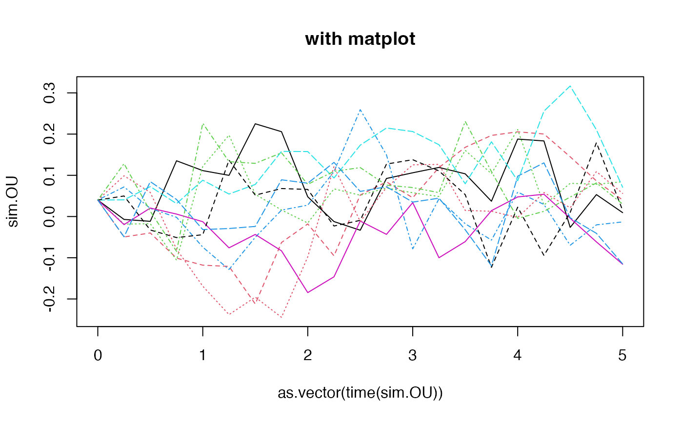
# OU

sim.OU <- simdiff(n = 10, horizon = 5, 
               frequency = "quart",  
               model = "OU", 
               x0 = V0, theta1 = theta1, theta2 = theta2, theta3 = theta3)
head(sim.OU)
#>          Series 1    Series 2    Series 3     Series 4   Series 5     Series 6
#> [1,]  0.040000000  0.04000000  0.04000000  0.040000000 0.04000000  0.040000000
#> [2,] -0.007010219 -0.04956433 -0.01826895  0.071842481 0.04048347 -0.019585761
#> [3,] -0.011615890 -0.03983938 -0.01748681  0.019752326 0.07264790  0.020593615
#> [4,]  0.135262514 -0.10092946 -0.10564592 -0.001863971 0.03134923  0.005970775
#> [5,]  0.111386836 -0.11799548  0.12182156 -0.074206258 0.08810187 -0.012538258
#> [6,]  0.099907491 -0.12101413  0.19755359 -0.128389846 0.05456646 -0.075926539
#>         Series 7    Series 8    Series 9   Series 10
#> [1,]  0.04000000  0.04000000  0.04000000  0.04000000
#> [2,]  0.04986768  0.09886257  0.12829678 -0.04918709
#> [3,] -0.03268803  0.05846365  0.01268510  0.08465305
#> [4,] -0.05110350 -0.07917464 -0.08446948  0.04136244
#> [5,] -0.04409434 -0.16895107  0.22629756 -0.03165900
#> [6,]  0.13685786 -0.23793961  0.13307614 -0.02906855
#par(mfrow=c(2,1))
esgplotbands(sim.OU, xlab = "time", ylab = "values", main = "with esgplotbands")                

matplot(as.vector(time(sim.OU)), sim.OU, type = 'l', main = "with matplot")                



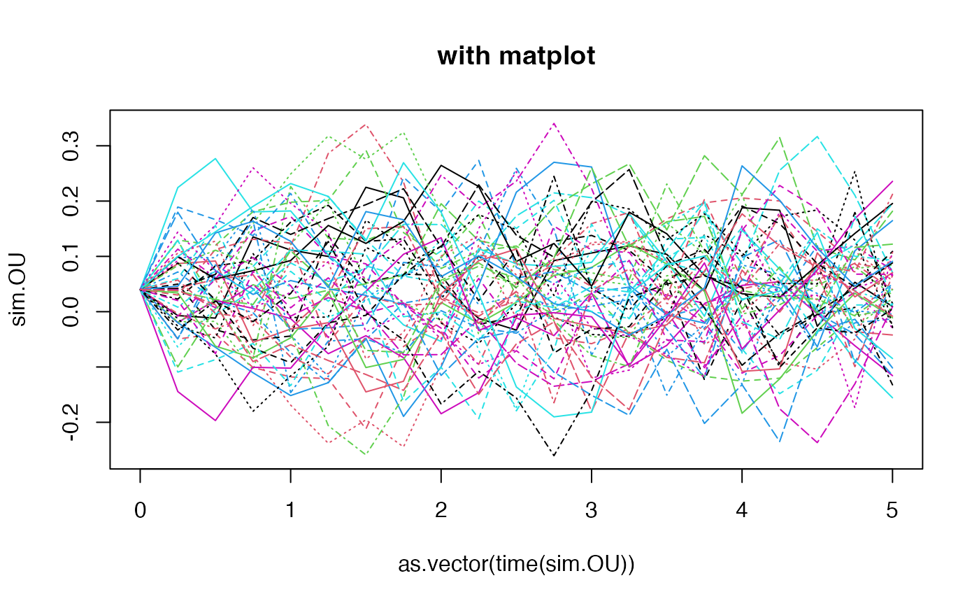
# OU with simulated shocks (check the dimensions)

eps0 <- simshocks(n = 50, horizon = 5, frequency = "quart", method = "anti")
sim.OU <- simdiff(n = 50, horizon = 5, frequency = "quart",   
               model = "OU", 
               x0 = V0, theta1 = theta1, theta2 = theta2, theta3 = theta3, 
               eps = eps0)
#par(mfrow=c(2,1))
esgplotbands(sim.OU, xlab = "time", ylab = "values", main = "with esgplotbands")                

matplot(as.vector(time(sim.OU)), sim.OU, type = 'l', main = "with matplot")

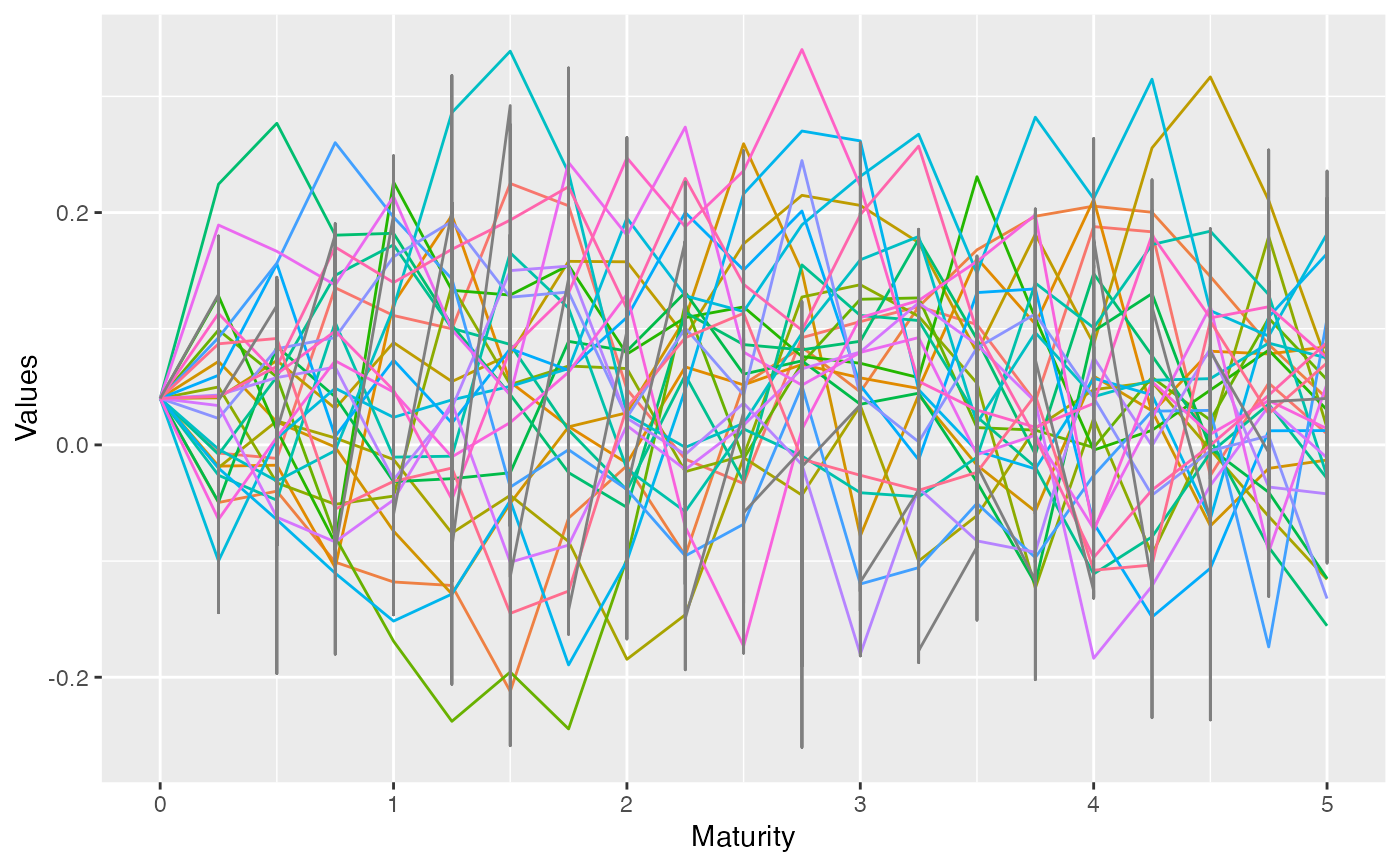
# a different plot
esgplotts(sim.OU)
#> Warning: Use of `meltdf$value` is discouraged.
#> ℹ Use `value` instead.



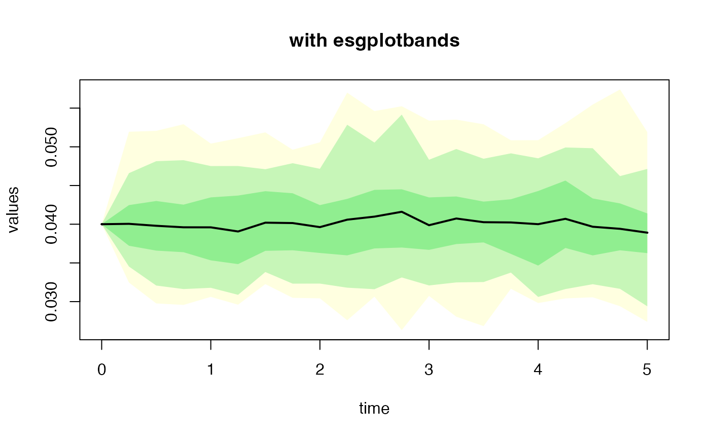
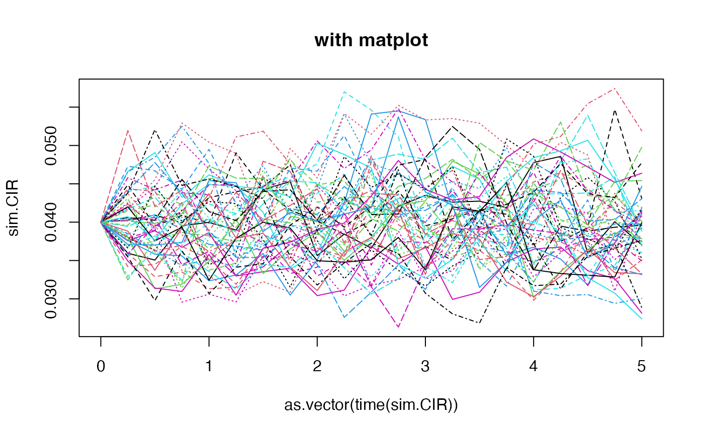
# CIR

sim.CIR <- simdiff(n = 50, horizon = 5, 
               frequency = "quart",  
               model = "CIR", 
               x0 = V0, theta1 = theta1, theta2 = theta2, theta3 = 0.05)
esgplotbands(sim.CIR, xlab = "time", ylab = "values", main = "with esgplotbands")                  

matplot(as.vector(time(sim.CIR)), sim.CIR, type = 'l', main = "with matplot")




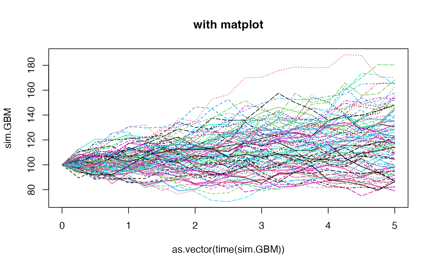
# GBM

eps0 <- simshocks(n = 100, horizon = 5, frequency = "quart")
sim.GBM <- simdiff(n = 100, horizon = 5, frequency = "quart",   
               model = "GBM", 
               x0 = 100, theta1 = 0.03, theta2 = 0.1, 
               eps = eps0)
esgplotbands(sim.GBM, xlab = "time", ylab = "values", main = "with esgplotbands")                

matplot(as.vector(time(sim.GBM)), sim.GBM, type = 'l', main = "with matplot")



eps0 <- simshocks(n = 100, horizon = 5, frequency = "quart")
sim.GBM <- simdiff(n = 100, horizon = 5, frequency = "quart",   
               model = "GBM", 
               x0 = 100, theta1 = 0.03, theta2 = 0.1, 
               eps = eps0)                
esgplotbands(sim.GBM, xlab = "time", ylab = "values", main = "with esgplotbands")                

matplot(as.vector(time(sim.GBM)), sim.GBM, type = 'l', main = "with matplot")




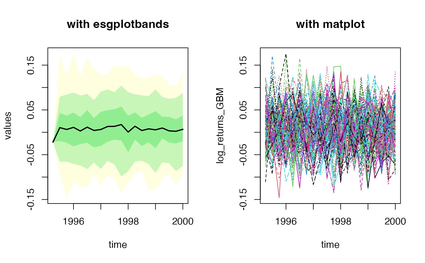
# GBM log returns (haha) with starting date 

eps0 <- simshocks(n = 100, horizon = 5, frequency = "quart", start = c(1995, 1))
sim.GBM <- simdiff(n = 100, horizon = 5, frequency = "quart",   
               model = "GBM", 
               x0 = 100, theta1 = 0.03, theta2 = 0.1, 
               eps = eps0, start = c(1995, 1))
log_returns_GBM <-  calculatereturns(sim.GBM, type = "log")  
par(mfrow=c(1, 2))
esgplotbands(log_returns_GBM , xlab = "time", ylab = "values", main = "with esgplotbands")
matplot(as.vector(time(log_returns_GBM)), log_returns_GBM, type = 'l', 
main = "with matplot", xlab = "time")

Arguments

Value

References

See also

Author

Examples